
Clark-Evans index allows you to define the way points are distributed in space – by chance, evenly or by group clustering. Earlier there was a post about this index at 50º North. It described in detail the theoretical aspects of calculating Clark-Evans index and its interpretation. Therefore, now we will not look into them again. In this post we draw attention to the practical aspects. Previously, we wrote about working with Clark-Evans test in ArcGIS. This time we will get acquainted with this test in R.
R is a programming language and also an environment for statistical calculations. It implements all standard statistical analysis procedures. There are also many additional packages with features that allow you to solve various specialized tasks, including those in the field of spatial statistics.
The history of R begins in 1996 in New Zealand. Two scientists from the University of Auckland, Ross Ihaka and Robert Gentleman, created it as a free analogue of S-Plus. The main benefits of R are that it is free and open source. Thoughout its existence, R has gained such popularity that now it can be called the favorite programming language of professional statisticians. In fact, in our opinion, it is turning into a professional standard in the field. As a result, R is often updated. All the latest achievements of statistics immediately appear in it as additional packages, the number of which already goes to thousands. Therefore, it is not an exaggeration to say that R is more superior than all commercial statistical programs that exist today.
Although, one drawback of R for many users is the relative complexity of learning to work with it. One has to work in command line mode. Now there are graphical user interfaces, such as RCommander, RKWard, and others. But they implement standard statistical analysis procedures. To work with the criteria of spatial statistics, you need to be able to write the code in R. And we want to show that it is not as difficult as it can initially give up.
This post begins a whole series on spatial statistics in the context of R environment. Like the next posts in this series, it will work better for those who have basic skills in R. If you do not already have them, you can refer to textbooks and online courses. We will focus on the functions necessary to calculate the criteria of spatial statistics. But if possible, we will also briefly describe the basic functions as well. In order to facilitate reading, the names of the packages, functions, objects and all the elements of the code will be highlighted. Separately, in the text of the post will be given the code snippets. In these fragments, the code elements will be marked in different colors. Functions are marked with blue, the function’s name is dark green, the object names are orange, the remaining elements – black.
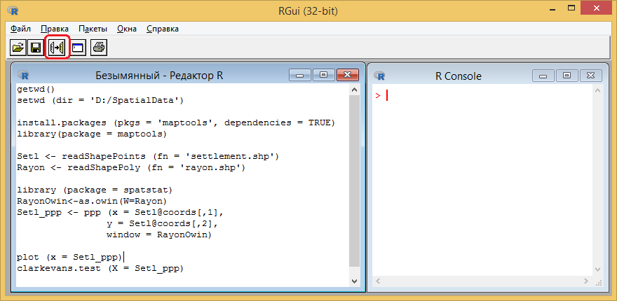
The whole code in R, which we will analyze in this post, is shown in Figure 1. This figure shows R interface. The left-hand side contains the code, and to the right is the console. To run the code, it is necessary to select a code snippet in the code editor and click on the button that is marked in figure 1. After that the result will appear in the console. You can also enter the code directly into the console and launch it by pressing the Enter button on the keyboard.
Fig. 1. R interface
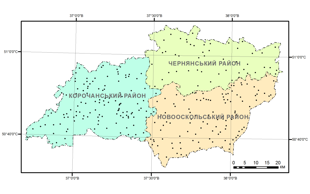
Calculation of the Clark-Evans index in R is performed using an example analysis of the population distribution. The data for the analysis are shown in Figure 2. These are cities, villages, settlements and farms in the three districts located in the Belgorod region – Korochansky, Novoosskolsky and Chernyansky districts.
Fig. 2. Settlements in the study area
1. Importing shape-files into R
For Clark-Evans test in R, you can use vector spatial data in a shapefile format as the primary data source. You must have two files. One of them is a shape with point geometry, for which it is necessary to perform the Clark-Evans test. The second one is a shape with a polygonal geometry that outlines the boundaries of the studied area. It is needed to estimate the area of this territory. In our example, we use files under the names settlement.shp (locations of settlements) and rayon.shp (administrative area).
There are different ways to import the shapefiles into R environment. We will implement it using the maptools package. This package contains functions for reading and processing spatial data.
1) To import shapes, first we set the working directory from which we will import the data. To find out which folder is the default one, you need to start the getwd function. No arguments need to be specified for it.
getwd()
After running the getwd function, the path to the working folder will be displayed in the console. If this folder is convenient for you, then you need to copy the shapes to it and proceed to import them into R. Be careful to copy all the file parts with the same name and different extensions (shp, shx, dbf and others, read more here), otherwise a part of the information may be lost or, in general, the shape file cannot be read.
If you want to choose another folder, make it the default one using the setwd function. It has one argument – dir. It specifies the path to the working folder (it should be written with the quotation marks).
setwd (dir = ‘D:/SpatialData’)
Pay attention to the slash sign that is in the path to the working folder. In R it is necessary to use a backslash.
2) The maptools package is one of R’s additional packages. That is, it is not a part of R by default, it needs to be installed separately using the install.packages function, which loads the package from the Internet and installs it in R’s program folder. The pkgs argument is the package name. If the dependencies argument is set to TRUE, the program installs not only the maptools package, but also other packages that are required for it to work.
install.packages (pkgs = 'maptools', dependencies = TRUE)
If the package is already installed on the computer, you must start it. Some packages run on R startup automatically. But all additional packages must be started manually. To do this, use the library function. Its package argument is the name of the package (no quotation marks necessary).
library (package = maptools)
3) After you start the maptools package, you can import shapefiles into R. To do this, the functions readShapePoints and readShapePoly are assigned in maptools. The first function imports shapes with point geometry, and the second one – polygonal geometry. The name of the file we import for the both functions is set by the fn argument.
Each shapefile is written to a separate object (a layer with settlements into the Setl object, and a layer with work area boundary – into Rayon object). To do this, we first write the name of the object, then the assignment symbol (<-), and then the function itself.
Setl <- readShapePoints (fn = 'settlement.shp')
Rayon <- readShapePoly (fn = 'rayon.shp')
The maptools package works with specific object classes. For spatial spatial data, this is a SpatialPointDataFrame class. For polygon data it is a SpatialPoligonDataFrame class. However, the spatstat package does not work with these object classes. Therefore, it is necessary to convert the data into objects of other classes. For point objects in spatstat there is a ppp class. And the boundaries of the study area are indicated by an object of the owin class.
2. Create an owin class object
For point data spatial analysis R has the spatstat package. This is also an additional package, like maptools. And it also needs to be run manually using the library function.
library (package = spatstat)
First, you need to create an owin class object, and then an object of ppp class. Because owin is used in the ppp creation process. In our example, we convert Rayon object to owin. To do this, there is an as.owin function. Its W argument is the object from which we make the owin class object.
RayonOwin <- as.owin(W = Rayon)
3. Create a ppp class object
The spatstat package works with a special class of objects – ppp. Objects of this class are created using a function that is also called ppp. For our example, we set values for the three arguments of this function. The arguments x and y are two vectors with the coordinates of the points (respectively, X and Y coordinates in the rectangular coordinate system). The window argument is the boundary of the area we explore. To add point coordinates, we will use the Setl object, which we created from the settlement.shp shapefile. This ppp class property contains point coordinate information. But you need to know how to read it.
The ppp class object is a complex object. It consists of separate parts (slots). To read the information from a slot, you need to write and run this code without spaces – the name of the object, the @ sign, the name of the slot. A slot containing coordinate information in any object in the ppp class is called coords.
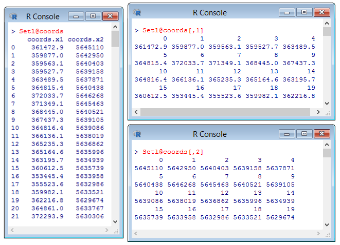
The first line of the code shown below displays the coordinates X and Y together in two columns in the console. The result of its implementation is shown in Figure 3 on the left. To access a single column, you need to add a column number to this code (without spaces) in square brackets. An example of this is the second line of the code below.
Column number 1 is the X coordinate, column number 2 is the Y coordinate. Note that there is a comma before the column number. It separates the row number from the column number. In our case, we do not address any single row, but all the rows of the selected column. Therefore, there is no need to write the line number, but you still have to put a comma.
Setl@coords
Setl@coords[,1]
Приклад виведення координат у консоль R показаний на рисунку 3.
Fig. 3. Coordinates in the R console (on the left – both coordinates, X and Y, on the right from the top – X, to the right below – Y)
As the value for the window argument you can specify an object of owin class. In our case, this is RayonOwin object.
Setl_ppp <- ppp (x = Setl@coords[,1],
y = Setl@coords[,2],
window = RayonOwin)
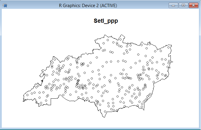
Once we have created a ppp object, it can be represented graphically (Figure 4). Although, it is better to make cartographic images in a GIS. In R, use the visualization only to verify that the object is created correctly.
plot (x = Setl_ppp)
Fig. 4. Result of rendering object of class ppp
If everything is done correctly, we will see all points with the same spatial arrangement that was in the shapefile. The boundary of the study area will delineate the points. Compare Figure 2 and Figure 4, and you will see that in our example everything is in its place.
4. Performing the Clark-Evans test
When our ppp class object is created, we can finally complete the Clark-Evans test. It is done using the clarkevans.test function. Its X argument is the name of the object of the ppp class for which we perform the test.
clarkevans.test (X = Setl_ppp)
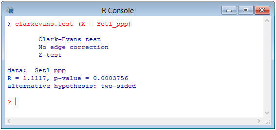
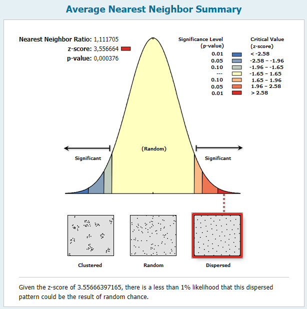
After running clarkevans.test, the console will contain values of the Clark-Evans index and the p-value. For our example, the Clark-Evans (R) criterion is approximately 1.11, which is statistically significantly greater than 1.00 (p <0.05). These results show that the settlements in the Korochansky, Novosskolsky and Chernianskyi districts are distributed uniformly in space (Fig. 5).
Fig. 5. The Clark-Evans test result in the R console (above) and the result of the test obtained using ArcGIS (below)
If we compare the results obtained with R and ArcGIS, then we see that they are the same. But in R there are options for calculating the Clark-Evans index, which are absent in ArcGIS. But we will look into that in a separate post.



Hi, thanks a lot. This blog helped me perform Clark-Evans test in R. Your step-by-step explanations was very useful.